Math 514 – Midterm Review Dec 12, 2018 Shawn Math 514 No comments yet Math 514 – Ch 5 Oct 10, 2018 Shawn Math 514 No comments yet Math 514 – Ch 4 Oct 03, 2018 Shawn Math 514 No comments yet Math 514 – Ch 3 Oct 01, 2018 Shawn Math 514 No comments yet Math 514 – Norm & Condition Number Sep 26, 2018 Shawn Math 514 1 comment 1 2 3 4
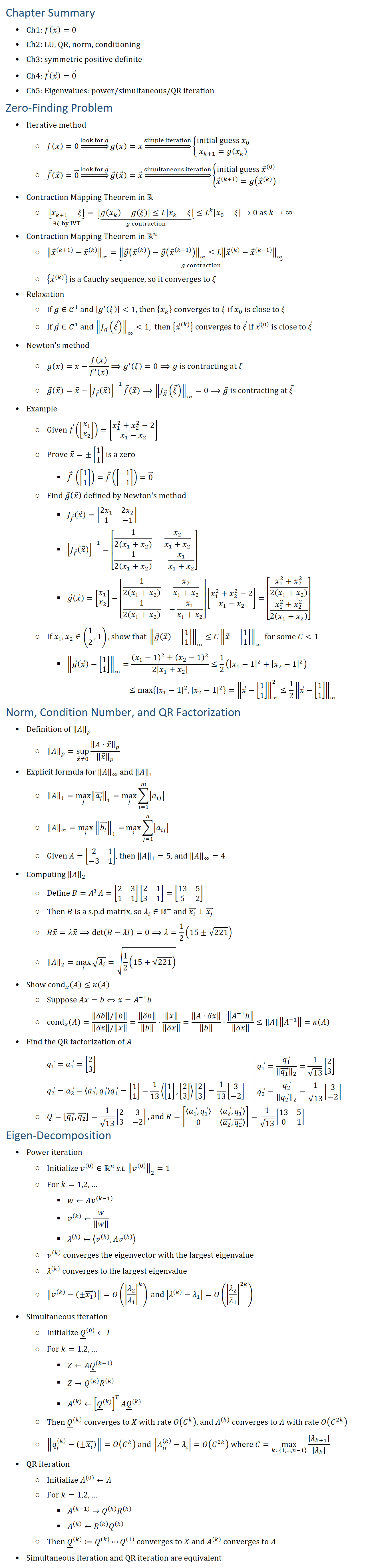

![Symmetric Positive Definite Matrix • Definition ○ Matrix A is called symmetric positive definite (s.p.d) if ○ A=A^T (symmetric) ○ x^T Ax0,∀x∈R(n×n)∖{0} (positive definite) • Proof: a_ii0 ○ a_ii=e_i^T Ae_i0, where [e_i ]_k={■8(1&if k=i@0&if k≠i)┤ • Proof: λ_i∈R+ for Ax_i=λ_i x_i ○ Use (λ_i ) ̅ to denote the conjugate of λ_i, we first need to show that (λ_i ) ̅=λ_i ○ Taking conjugate on both sides of Ax_i=λ_i x_i, we obtain A(x_i ) ̅=(λ_i ) ̅(x_i ) ̅ (note: A=A ̅) ○ {█(&x_i^T A(x_i ) ̅=x_i^T ((λ_i ) ̅(x_i ) ̅ )=(λ_i ) ̅x_i^T (x_i ) ̅@&x_i^T A(x_i ) ̅=┴sym x_i^T A^T (x_i ) ̅=(Ax_i )^T (x_i ) ̅=λ_i x_i^T (x_i ) ̅ )┤⇒(λ_i ) ̅x_i^T (x_i ) ̅=λ_i x_i^T (x_i ) ̅⇒(λ_i ) ̅=λ_i⇒λ_i∈R ○ x_i^T Ax_i=λ_i x_i^T x_i⇒λ_i=(x_i^T Ax_i)/(x_i^T x_i )0, since x_i^T Ax_i0 and x_i^T x_i0 ○ Note: λ_i∈R holds for all symmetric matrices • Proof: ⟨x_i,x_j ⟩=0 for λ_i≠λ_j ○ {█(&x_i^T Ax_j=x_i^T (λ_j x_j )=λ_j x_i^T x_j@&x_i^T A^T x_j=(Ax_i )^T x_j=λ_i x_i^T x_j )┤⇒(λ_j−λ_i ) x_i^T x_j=0 ○ If λ_i≠λ_j, then x_i^T x_j=⟨x_i,x_j ⟩=0 • Proof: det〖(A)0〗 ○ A[(x_1 ) ⃗, (x_2 ) ⃗,…,(x_n ) ⃗ ]=[λ_1 (x_1 ) ⃗,λ_2 (x_2 ) ⃗,…,λ_n (x_n ) ⃗ ]=[(x_1 ) ⃗, (x_2 ) ⃗,…,(x_n ) ⃗ ][■(λ_1&&&@&λ_2&&@&&⋱&@&&&λ_n )] ○ Let X=[(x_1 ) ⃗, (x_2 ) ⃗,…,(x_n ) ⃗ ], Λ=[■(λ_1&&&@&λ_2&&@&&⋱&@&&&λ_n )], then AX=XΛ⇒A=XΛX^(−1) ○ Therefore, |A|=|XΛX^(−1) |=|X||Λ| |X|^(−1)=|Λ|=∏_(i=1)^n▒λ_i 0 • Proof: Let I⊊{1,2,…,n}, then B=A_II is also s.p.d. ○ A=A^T⇒A_II=A_II^T⇒B=B^T ○ Define y∈Rn s.t. [y]_i={■8([x]_i&i∈I@0&o.w.)┤, then x^T Bx=y^T Ay0,∀x∈R|I| ∖{0} • Cholesky Decomposition ○ If A is s.p.d., then ∃L lower diagonal s.t. A=LL^T ○ Note: This is saying that after LU decomposition, U=L^T Ordinary Differential Equation (Boundary Value Problem) • Suppose u(x)∈C^2 [0,1], find the solution for {█(u^′′+2u^′=−1@u(x=0)=0@u(x=1)=0)┤ • We can evenly sample N points on [0,1]: Δx=1/(N+1), x_i=iΔx • Compute first derivative u^′ (x_j ) using u(x_(j+1) ) and u(x_(j−1) ) ○ u^′ (x_j )=lim┬(δ→0)〖(u(x_j+δ)−u(x_j−δ))/2δ〗≈(u(x_(j+1) )−u(x_(j−1) ))/2Δx ○ Note: ├ Du┤|_j=(u(x_(j+1) )−u(x_(j−1) ))/2Δx is called the discrete derivative of u at j • Compute second derivative u^′′ (x_j ) using u(x_(j+2) ), u(x_j ) and u(x_(j−2) ) u^′′ (x_j )=lim┬(δ→0)〖(u^′ (x_j+δ)−u^′ (x_j−δ))/2δ〗 ≈(u^′ (x_(j+1) )−u^′ (x_(j−1) ))/2Δx ≈(((u(x_(j+2) )−u(x_j ))/2Δx)−((u(x_j )−u(x_(j−2) ))/2Δx))/2Δx, by substituting u^′ =(u(x_(j+2) )−2u(x_j )+u(x_(j−2) ))/(4Δx^2 ) • Compute second derivative u^′′ (x_j ) using u(x_(j+1) ), u(x_j ) and u(x_(j−1) ) ○ In practice, we want to only use neighboring points to have a local approximation ○ Thus, u^′′ (x_j )≈(u^′ (x_(j+1∕2) )−u^′ (x_(j−1∕2) ))/Δx=(u(x_(j+1) )−2u(x_j )+u(x_(j−1) ))/(Δx^2 ) • Substitute u^′,u^′′ into the ODE ○ (u(x_(j+1) )−2u(x_j )+u(x_(j−1) ))/(Δx^2 )+2((u(x_(j+1) )−u(x_(j−1) ))/2Δx)≈−1 ○ Define U≔[█(u(x_1 )@⋮@u(x_n ) )], then (U_(j+1)−2U_j+U_(j−1))/(Δx^2 )+(U_(j+1)−U_(j−1))/Δx=−1 ○ Let A∈R(n×n) s.t. [A]_ij={■8((Δx^2 )^(−1)−(Δx)^(−1)&i=j−1@−2(Δx^2 )^(−1)&i=j@(Δx^2 )^(−1)+(Δx)^(−1)&i=j+1@0&o.w.)┤, then AU=−1 ○ Note: A is said to be a tri-diagonal matrix [■(∗&∗&&&@∗&∗&∗&&@&∗&∗&∗&@&&∗&∗&∗@&&&∗&∗)]](https://shawnzhong.com/wp-content/uploads/2018/10/img_5bb4eee9117a8.png)
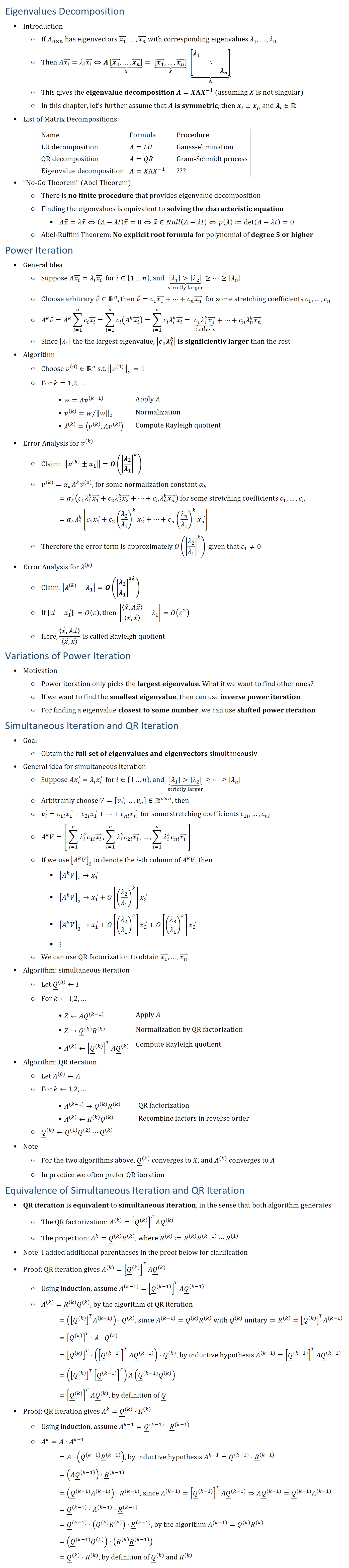
![Norm (Definition 2.6) • Let V be a linear space, and ‖⋅‖: V→R(≥0) • ‖⋅‖ is said to be a norm if ○ ‖v ⃗ ‖=0⇔v=0 (positive definite) ○ ‖αv ⃗ ‖=|α|‖v ⃗ ‖ ○ ‖v ⃗+w ⃗ ‖≤‖v ⃗ ‖+‖w ⃗ ‖ (triangle inequality) Vector Norm (Definition 2.7 & 2.8 & 2.9) • 2-norm (Euclidean norm) ○ ‖v ⃗ ‖_2≔√(v_1^2+…+v_n^2 )=√(∑_(i=1)^n▒v_i^2 ) • 1-norm (taxicab norm / Manhattan norm) ○ ‖v ⃗ ‖_1≔|v_1 |+…+|v_n |=∑_(i=1)^n▒|v_i | ○ In order to show that 1-norm is a valid norm, we still need to prove § ‖v ⃗+w ⃗ ‖_1=∑_(i=1)^n▒|v_i+w_i | ≤∑_(i=1)^n▒〖|v_i |+|w_i | 〗=‖v ⃗ ‖_1+‖w ⃗ ‖_1 • ∞-norm (maximum norm) ○ ‖v ⃗ ‖_∞≔max┬(i∈{1,…,n} )|v_i | • p-norm, for p≥1 ○ ‖v ⃗ ‖_p≔(∑_(i=1)^n▒|v_i^p | )^(1∕p) ○ Minkowski’s inequality § ‖u ⃗+v ⃗ ‖_p≤‖u ⃗ ‖_p+‖v ⃗ ‖_p § This proves the triangle inequality for p-norm Matrix Norm (Definition 2.10) • Given a matrix A_(m×n)=[■8(a_11&⋯&a_1n@⋮&⋱&⋮@a_m1&…&a_mn )] • Frobenius norm ○ ‖A‖_F≔√(∑_(i=1)^m▒∑_(j=1)^n▒a_(i,j)^2 ) ○ The matrix is viewed as a list of number • Operator norm / induced norm ○ ‖A‖_(p,q)≔sup_(x ⃗∈Rn∖{0 ⃗ } )〖‖Ax ⃗ ‖_q/‖x ⃗ ‖_p 〗 ○ The matrix is viewed as a linear transformation ○ Operator norm is a means to measure the "size" of linear operators ○ Note that the operator norm has two parameter p and q • In particular, if both parameters equal to p, we simply call it p-norm ○ ‖A‖_p≔sup_(x ⃗∈Rn∖{0 ⃗ } )〖‖Ax ⃗ ‖_p/‖x ⃗ ‖_p 〗 ○ 1-norm, 2-norm and ∞-norm are defined similarly • Triangle inequality for p-norm ○ Without loss of generality, suppose ‖x ⃗ ‖_p=1 ○ ‖(A+B) x ⃗ ‖_p=‖Ax ⃗+Bx ⃗ ‖_p≤‖Ax ⃗ ‖_p+‖Bx ⃗ ‖_p ○ ⇒‖(A+B) x ⃗ ‖_p/‖x ⃗ ‖_p ≤‖Ax ⃗ ‖_p/‖x ⃗ ‖_p +‖Bx ⃗ ‖_p/‖x ⃗ ‖_p ○ ⇒‖A+B‖_p≤‖A‖_p+‖B‖_p • ‖AB‖_p≤‖A‖_p ‖B‖_p ○ ‖ABx ⃗ ‖_p≤‖A‖_p ‖Bx ⃗ ‖_p≤‖A‖_p ‖B‖_p ‖x ⃗ ‖_p ○ ‖ABx ⃗ ‖_p/‖x ⃗ ‖_p ≤‖A‖_p ‖B‖_p ○ ‖AB‖_p≤‖A‖_p ‖B‖_p ‖A‖_1=Maximum Absolute Column Sum (Theorem 2.8) • Statement ○ Given a matrix A_(n×m)=[(a_1 ) ⃗,…,(a_n ) ⃗ ], then ○ ‖A‖_1=sup_(x ⃗∈Rn∖{0 ⃗ } )〖‖Ax ⃗ ‖_1/‖x ⃗ ‖_1 〗=max┬(j∈{1,…,n} )〖‖(a_j ) ⃗ ‖_1 〗=(max)┬(j∈{1,…,n} )∑_(i=1)^m▒|a_ij | • Note ○ The 1-norm of matrix is also called maximum absolute column sum • Proof ○ Let C≔max┬(j∈{1,…,n} )〖‖(a_j ) ⃗ ‖_1 〗=max┬(j∈{1,…,n} )∑_(i=1)^m▒|a_ij | ○ Show that ‖Ax ⃗ ‖_1≤C‖x ⃗ ‖_1,∀x∈Rn∖{0 ⃗ } § ‖Ax ⃗ ‖_1=∑_(i=1)^m▒|(Ax ⃗ )_i | , by definition of 1\-norm of vector § =∑_(i=1)^m▒|∑_(j=1)^n▒〖a_ij x_j 〗| , by definition of Ax ⃗ § ≤∑_(i=1)^m▒∑_(j=1)^n▒|a_ij ||x_j | , by triangle inequality § =∑_(j=1)^n▒(∑_(i=1)^m▒|a_ij | )|x_j | , since only |a_ij | depends on i § ≤C∑_(j=1)^n▒|x_j | , by maximality of C § =C‖x ⃗ ‖_1, by definition of 1\-norm of vector ○ Look for an x ⃗ s.t. ‖Ax ⃗ ‖_1=C‖x ⃗ ‖_1 § Let J≔(argmax)┬(j∈{1,…,n} )〖‖(a_j ) ⃗ ‖_1 〗, then ‖(a_J ) ⃗ ‖_1=C § Let x ⃗∈Rn s.t. [x ⃗ ]_k={■8(1&k=J@0&k≠J)┤, then ‖x ⃗ ‖_1=1 § Therefore ‖Ax ⃗ ‖_1=‖(a_J ) ⃗ ‖_1=C=C‖x ⃗ ‖_1 ‖A‖_∞=Maximum Absolute Row Sum (Theorem 2.7) • Statement ○ Given a matrix A_(n×m)=[█((b_1 ) ⃗@⋮@(b_m ) ⃗ )], then ○ ‖A‖_∞=sup_(x ⃗∈Rn∖{0 ⃗ } )〖‖Ax ⃗ ‖_∞/‖x ⃗ ‖_∞ 〗=max┬(i∈{1,…,m} )〖‖(b_i ) ⃗ ‖_∞ 〗=(max)┬(i∈{1,…,m} )∑_(i=1)^m▒|a_ij | • Note ○ The ∞-norm of matrix is also called maximum absolute row sum • Proof ○ Let C≔max┬(i∈{1,…,m} )〖‖(b_i ) ⃗ ‖_∞ 〗=max┬(i∈{1,…,m} )∑_(j=1)^n▒|a_ij | ○ Show that ‖Ax ⃗ ‖_∞≤C‖x ⃗ ‖_∞,∀x∈Rn∖{0 ⃗ } § ‖Ax ⃗ ‖_∞=max┬(i∈{1,…,m} )|∑_(j=1)^n▒〖a_ij x_j 〗|, by definition of ∞\-norm § ≤max┬(i∈{1,…,m} )∑_(j=1)^n▒|a_ij ||x_j | , by the triangle inequality § ≤[max┬(i∈{1,…,m} )∑_(j=1)^n▒|a_ij | ] ‖x ⃗ ‖_∞, by definition of ∞\-norm § =C‖x ⃗ ‖_∞ ○ Look for an x ⃗ s.t. ‖Ax ⃗ ‖_∞=C‖x ⃗ ‖_∞ § Let I=argmax┬(i∈{1,…,m} )〖‖(b_i ) ⃗ ‖_1 〗, then ‖(b_I ) ⃗ ‖_1=∑_(j=1)^n▒|a_Ij | =C § Let x ⃗∈Rn s.t. [x ⃗ ]_j={■8(1&b_Ij0@−1&b_Ij<0)┤, then ‖x ⃗ ‖_∞=1 § Then [Ax ⃗ ]_I=(b_I ) ⃗^T x ⃗=|∑_(j=1)^n▒〖a_Ij x_j 〗|=∑_(j=1)^n▒|a_Ij | =C=C‖x ⃗ ‖_∞ ‖A‖_2=Largest Singular Value (Theorem 2.9) • Positive-definite ○ A matrix A is said to be positive-definite if ○ All its eigenvalues are positive, and all the eigenvector is orthonormal ○ i.e. λ_i∈R+ and {█(‖(x_i ) ⃗ ‖_2=1@x_i⊥(x_j ) ⃗ )┤⇒⟨(x_i ) ⃗,(x_j ) ⃗ ⟩=δ_ij={■8(1&i=j@0&i≠j)┤ for A(x_i ) ⃗=λ_i (x_i ) ⃗ • Symmetric ○ A matrix A is said to be symmetric if A^T=A • Statement (special case) ○ Assume A_(n×n) is a positive-definite symmetric matrix ○ Then ‖A‖_2=sup_(x ⃗∈Rn∖{0 ⃗ } )〖‖Ax ⃗ ‖_2/‖x ⃗ ‖_2 〗=(max)┬(i∈{1,…,n} )|λ_i | • Proof (for special case) ○ Let C=sup_(x ⃗∈Rn∖{0 ⃗ } )〖‖Ax ⃗ ‖_2/‖x ⃗ ‖_2 〗 ○ Show C≤max┬(i∈{1,…,n} )|λ_i | § Express x ⃗ as a linear combination of the orthonormal vectors {x_i } □ x ⃗=c_1 (x_1 ) ⃗+c_2 (x_2 ) ⃗+…+c_n (x_n ) ⃗ □ Then ‖x ⃗ ‖_2=√(∑c_i^2 ) § Similarly, express Ax ⃗ using {x_i } □ Ax ⃗=c_1 A(x_1 ) ⃗+c_2 A(x_2 ) ⃗+…+c_n A(x_n ) ⃗ =c_1 λ_1 (x_1 ) ⃗+c_2 λ_2 (x_2 ) ⃗+…+c_n λ_n (x_n ) ⃗ □ Then ‖Ax ⃗ ‖_2=√(∑▒〖c_i^2 λ_i^2 〗) § Thus, ‖Ax ⃗ ‖_2/‖x ⃗ ‖_2 ≤√((∑▒〖c_i^2 λ_i^2 〗)/(∑▒c_i^2 ))≤max┬(i∈{1,…,n} )|λ_i |,∀x ⃗∈Rn∖{0 ⃗ } ○ Look for an x ⃗ s.t. ‖Ax ⃗ ‖_2=C‖x ⃗ ‖_2 § Let I=(argmax)┬(i∈{1,…,n} )|λ_i |, then |λ_I |=C § Let x ⃗=(x_I ) ⃗, then ‖Ax ⃗ ‖_2/‖x ⃗ ‖_2 =‖A(x_I ) ⃗ ‖_2/‖(x_I ) ⃗ ‖_2 =√((c_I^2 λ_I^2)/(c_I^2 ))=|λ_I |=C=C‖x ⃗ ‖_2 • Statement (General Case) ○ Define B_(n×n)=A_(n×m)^T A_(m×n), then B is a positive-definite symmetric matrix ○ Let S_i=√(λ_i ), then S_i is called the singular values of A ○ The previous statement can be generalized to ‖A‖_2=(max)┬(i∈{1,…,n} )|S_i | Conditioning of Function (Example 2.5 & 2.6) • Motivation ○ Suppose the input x has a perturbation of τ (because of machine percision) ○ Wed like to know how the output f will be affected by τ ○ Conditioning is used to measure the sensitivity of the output to perturbations in the input • Absolute conditioning ○ Cond(f)=(sup)┬█(x,y∈D@x≠y)〖|f(x)−f(y)|/|x−y| 〗 ○ If f is differentiable, then Cond(f)=(sup)┬(x∈D)|f^′ (x)| • Absolute local conditioning ○ Cond_x (f)=(sup)┬█(|δx|→0@x+δx∈D)〖|f(x+δx)−f(x)|/|δx| 〗 ○ If f is differentiable, then Cond_x (f)={■8(|f^′ (x)|&if f is a scalar function@|∇f(x)|&if f is a vector function)┤ • Relative local conditioning ○ Cond_x (f)=sup┬█(|δx|→0@x+δx∈D)〖(|f(x+δx)−f(x)|∕|f(x)| )/(|δx|∕|x| )〗=sup┬█(|δx|→0@x+δx∈D)〖|f(x+δx)−f(x)|/|δx| 〗⋅|x|/|f(x)| ○ If f is differentiable, then Cond_x (f)=|f^′ (x)|/|f(x)| |x| ○ Motivation § f(x)=1, f(x+δx)=2 § g(x)=100, g(x+δx)=101 § Both f and g increased 1, but the effects are different! • Example: f(x)=√x ○ Absolute § If D=[0,1], then Cond(f)=+∞ § If D=[1,2], then Cond(f)=1/2 ○ Absolute local § Cond_x (f)=f^′ (x)=1/(2√x)→{■8(∞ (ill-conditioned)&as x→0@0 (well-conditioned)&as x→+∞)┤ ○ Relative local § Cond_x (f)=|f^′ (x)|/|f(x)| |x|=(1∕(2√x) )/√x |x|=1/2,∀x∈D Condition Number of Matrix (Definition 2.12) • Definition ○ κ(A)=‖A‖‖A^(−1) ‖ is called the condition number of A ○ If κ(A)≫1, then we say A is ill-conditioned • Note ○ κ(A)=κ(A^(−1) ) ○ κ(A)≥1 • ▭(x(+δx) ) ⟶┴A ▭(b(+δb) ) ○ {█(Ax=b@A(x+δx)=b+δ(b) )┤⇒δb=Aδx ○ Cond_x (A)=(‖δb‖∕‖b‖ )/(‖δx‖∕‖x‖ ), by definition =‖δb‖/‖b‖ ⋅‖x‖/‖δx‖ =‖Aδx‖/‖Ax‖ ⋅‖x‖/‖δx‖ , since δb=Aδx and b=Ax =‖Aδx‖/‖δx‖ ⋅‖A^(−1) b‖/‖b‖ , assuming A is not singular ≤‖A‖‖A^(−1) ‖ by definition of matrix norm • ▭(A(+δA) ) →┴b ▭(x(+δx) ) ○ Ax=b ○ Ax=(A+δA)(x+δx), since b is viewed as the function here ○ Ax=Ax+δAx+Aδx+ ⏟δAδx┬(≈0), since δAδx is a second order turbulence ○ δAx+Aδx=0 ○ δx=−A^(−1)⋅δA⋅x ○ ‖δx‖≤‖A^(−1) ‖‖δA‖‖x‖, since ‖PQ‖≤‖P‖‖Q‖ for any matrix P,Q ○ (‖δx‖/‖x‖)/(‖δA‖/‖A‖ )=‖δx‖/‖x‖ ⋅‖A‖/‖δA‖ ≤‖A^(−1) ‖‖δA‖‖x‖/‖x‖ ‖A‖/‖δA‖ =‖A^(−1) ‖‖A‖ • We can similarly analyze ▭(b(+δb) ) ⟶┴A ▭(x(+δx) ) and ▭(A(+δA) ) →┴x ▭(b(+δb) ) • Note: The choice of norm will affect the condition number ○ A=[■(1&&&@1&1&&@⋮&&⋱&@1&&&1)]⇒A^(−1)=[■(1&&&@−1&1&&@⋮&&⋱&@−1&&&1)] ○ {█(‖A‖_∞=‖A^(−1) ‖_∞=2@‖A‖_1=‖A^(−1) ‖_1=n)┤⇒{█(Cond_(L_1 ) (A)=‖A‖_1 ‖A^(−1) ‖_1=n^2@Cond_(L_∞ ) (A)=‖A‖_∞ ‖A^(−1) ‖_∞=4)┤ Example for Condition Number • Let A=[■8(2&1@1&2)] • 1 norm • ∞ norm • 2 norm ○ S={[█(c@d)]=A[█(x@y)]│x^2+y^2=1} ○ Let A^(−1)=[■8(b_11&b_12@b_21&b_22 )], then [█(x@y)]=A^(−1) [█(c@d)]=[█(b_11 c+b_12 d@b_21 c+b_22 d)] ○ Since x^2+y^2=1, we have αc^2+βcd+γd^2=1, where § α=b_11^2+b_21^2 § β=2b_11 b_12+2b_21 b_22 § γ=b_12^2+b_22^2 ○ Since discriminant = β^2−4αγ<0, the graph S is an ellipse ○ κ(A)=(length of major axis)/(length of minor axis)=S_max/S_min , where S is the singular value Exercise 2.12 • Given ∃x s.t. (I−B)x=0 • Show ‖B‖_2=max┬(i=1…n)√(λ_i )≥1⇔∃λ_1≥1 ○ {█(x^T (I−B)x=x^T x−x^T Bx=0@x^T (I−B)^T (I−B)x=x^T x−2x^T Bx+x^T B^T Bx)┤⇒x^T B^T Bx=x^T x ○ ‖B‖_2=sup┬(x∈Rn∖{0} )〖‖Bx‖_2/‖x‖_2 〗=sup┬(x∈Rn∖{0} )√((x^T B^T Bx)/(x^T x))≥1 • Show (I−A)^(−1)=I+A(I−A)^(−1) ○ (I−A)(I+A(I−A)^(−1) )=(I−A)+A=I • Note: Neumann expansion ○ (I+A)^(−1)=I−A+A^2−A^3+⋯ ○ 1/(1+x)=1−x+x^2−x^3+⋯](https://shawnzhong.com/wp-content/uploads/2018/10/img_5bb4eea228b89.png)